Statistical Tolerance Analysis

Dimensional tolerances specify allowed variability around nominal dimensions. We assign tolerances to assure component interchangeability while meeting performance and producibility requirements. In general, as tolerances become smaller, manufacturing costs become greater. The challenge becomes finding ways to increase tolerances without sacrificing product performance and overall assembly conformance. Statistical tolerance analysis provides a proven approach for relaxing tolerances and reducing cost.
Before we dive into how to use statistical tolerance analysis, let’s first consider how we usually assign tolerances. Tolerances should be based on manufacturing process capabilities and requirements in the areas of component interchangeability, assembly dimensions, and product performance. In many cases, though, tolerances are based on an organization’s past tolerance practices, standardized tolerance assignment tables, or misguided attempts to improve quality by specifying needlessly-stringent tolerances. These latter approaches are not good; they often introduce fit and performance issues, and organizations that use them often leave money on the table.
There are two approaches to tolerance assignment: worst case tolerance analysis and statistical tolerance analysis.
In the worst case approach, we analyze tolerances assuming components will be at their worst case conditions. This seemingly innocuous assumption has several deleterious effects. It requires larger than necessary assembly tolerances if we simply stack the worst case tolerances. On the other hand, if we start with the required assembly tolerance and use it to determine component tolerances, the worst case tolerance analysis approach forces us to make the component tolerances very small. Here’s why this happens: The rule for assembly tolerance determination using the worst case approach is:
Tassy= ΣTi
where
Tassy = assembly tolerance
Ti = individual component tolerances
The worst case tolerance analysis and assignment approach assumes that the components will be at their worst case dimensions; i.e., each component will be at the extreme edge of its tolerance limits. The good news is that this is not a realistic assumption. It is overly conservative.
Here’s more good news: Component dimensions will most likely be normally distributed between the component’s upper and lower tolerance bounds, and the probability of actually being at the tolerance limits is low. The likelihood of all of the components in an assembly being at their upper and lower limits is even lower. The most likely case is that individual component dimensions will hover around their nominal values. This reasonable assumption underlies the statistical tolerance analysis approach. We can use statistical tolerance analysis to our advantage in three ways:
- If we start with component tolerances, we can assign a tighter assembly tolerance.
- If we start with the assembly tolerance, we can increase component tolerances.
- We can use combinations of the above two approaches to provide tighter assembly tolerances than we would use with the worst case tolerance analysis approach and to selectively relax component tolerances.
Statistical tolerance analysis uses a root sum square approach to develop assembly tolerances based on component tolerances. In the worst case tolerance analysis approach discussed above, we simply added all of the component tolerances to determine the assembly tolerance. In the statistical tolerance analysis approach, we find the assembly tolerance based on the following equation:
Tassy = (ΣTi2)(1/2)
Using the above formula is straightforward. We simply square each component tolerance, take the sum of these squares, and then find the square root of the summed squares to determine our assembly tolerance.
Consider this simple assembly with three parts, each with a tolerance of ±0.002 inch:
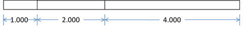
The worst case assembly tolerance for the above design is the sum of all of the component tolerances, or ±0.006 inch.
Using the statistical tolerance analysis approach yields an assembly tolerance based on the root sum square of the component tolerances. It is (0.0022 + 0.0022 + 0.0022)(1/2), or 0.0035 inch. Note that the statistically-derived tolerance is 42% smaller than the worst case tolerance. That’s a very significant decrease from the 0.006 inch worst case derived tolerance.
Based on the above, we can assign a tighter assembly tolerance while keeping the existing component tolerances. Or, we can stick with the worst case assembly tolerance (assuming this is an acceptable assembly tolerance) and relax the component tolerances. In fact, this is why we usually use the statistical tolerance analysis approach; for a given assembly tolerance, it allows us to increase the component tolerances (thereby lowering manufacturing costs).
Let’s continue with the above example to see how we can do this. Suppose we increase the tolerance of each component by 50% so that the component tolerances go from 0.002 inch to 0.003 inch. Calculating the statistically-derived tolerances in this case results in an assembly tolerance of 0.0052 inch, which is still below the 0.006 inch worst case assembly tolerance. This is very significant: We increased component tolerance 50% and still came in with an assembly tolerance less that the worst case assembly tolerance. We can even double one of the above component’s tolerances to 0.004 inch while increasing the other two by 50% and still lie within the worst case assembly tolerance. In this case, the statistically-derived assembly tolerance would be (0.0032 + 0.0032 + 0.0042)(1/2), or 0.0058 inch. It’s this ability to use statistical tolerance analysis to increase component tolerances that is the real money maker here.
The only disadvantage to the statistical tolerance analysis approach is that there is a small chance we will violate the assembly tolerance. An implicit assumption is that all of the components are produced using capable processes (i.e., the process capability is such that ±3σ or all parts produced lie within the tolerance limits for each part). This really isn’t much of an assumption (whether you are using statistical tolerance analysis or worst case tolerance analysis, your processes have to be capable). With a statistical tolerance analysis approach, we can predict that 99.73% (not 100%) of all assemblies will meet the required assembly dimension. This relatively small predicted rejection rate (just 0.27%) is usually acceptable. In practice, when the assembly dimension is not met, we can usually address it by simply selecting different components to bring the assembly into conformance.
If you’d like to learn more about statistical tolerance analysis and how to use it to reduce your manufacturing costs, check out the Eogogics workshops on Statistical Tolerance Analysis and Tolerance Stack Analysis Using GD&T. You will find additional, related courses listed at our Mechanical and Manufacturing Engineering Curriculum page. If you’d like to explore bringing one of these workshops to your company, please email us or call us at 1 (888) 364-6442.
Editor’s Note: Joe Berk, Principal Eogogics Faculty, possesses 30+ years of experience in engineering design. He teaches several of the Eogogics engineering courses including Statistical Tolerance Analysis, Unleashing Engineering Creativity, Poka-Yoke, Reliability Engineering, Root Cause Failure Analysis (RCFA), Process FMEA, Quality Management, Engineering Statistics, Design of Experiments, Statistical Process Control, Cost Reduction, Technical Management and Leadership, and Technical Communications. Before starting his training/consulting practice, he held senior management positions in engineering, quality assurance, and manufacturing. He’s the author of ten books on engineering. He holds undergraduate and graduate degrees in mechanical engineering from Rutgers University and an MBA from Pepperdine University.
Sorry, comments for this entry are closed at this time.