Digital Image Processing in Today’s Connected World

Tom Fowler, PhD

Photography — like audio, video, telephony, and most other forms of communication — went digital many years ago.  Digital images, whether from digital cameras, the Internet, or software programs, are used in nearly every industry as well as in science and technology, medicine, education, and many other areas.  Because the images are digital, a vast array of possibilities for manipulation and enhancement have opened up.  But while most people know the very basic principles of image manipulation, such as cropping, adjusting brightness and contrast, and some color adjustment, they do not have a firm grasp on all of the possibilities inherent in modern digital image processing, especially with high bit depth images.  This understanding is not necessary for most digital photography, since the automation in the cameras is sufficient to allow high-quality pictures with minimal user effort.  However when conditions become extreme, and equipment is pushed to its limits, an understanding of digital imaging and digital image processing at a deeper level becomes essential.  Such is typically the case in applications such as astronomy, geospatial work, medical imaging, microscopy, forensics, surveillance photography, in low-light and high-speed photography, and applications requiring reliable edge detection, such as robotics.

In this article, we will examine some techniques and typical applications of modern digital image processing.  A good understanding of the basics of pixilation and light is important for knowing how to deal with noise, and the fundamental limits of imaging systems, especially in areas such as resolution.  Most of the illustrations are drawn from astronomy, but the same techniques are used in nearly all application areas.

Extracting the Information

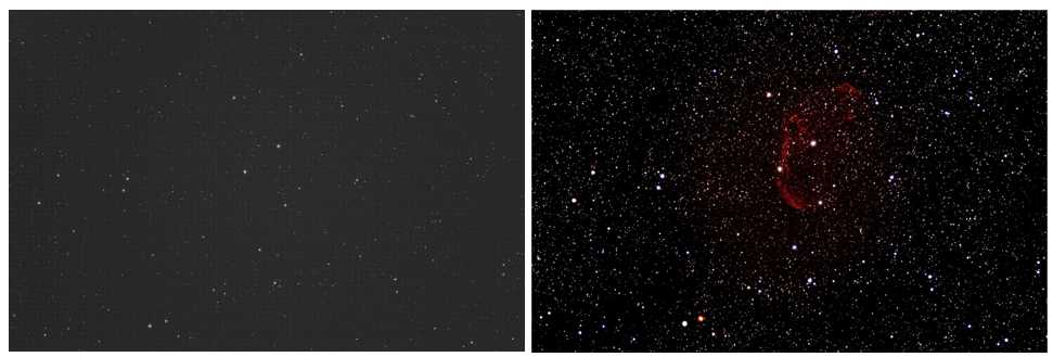
One of the goals of digital image processing is to extract information from images that do not seem to have it.  Histograms, for example, provides the basis for knowing how to extract images with very slight contrast differences.  For instance, how does one go from the image on the left to the one on the right?

To do this, one needs a solid understanding of histograms and how to use them to manipulate digital images.  A histogram is simply a plot of brightness level vs number of pixels with that brightness. The example below shows the histogram (left) for the image on the right. This histogram was generated by the excellent freeware app ImageJ.

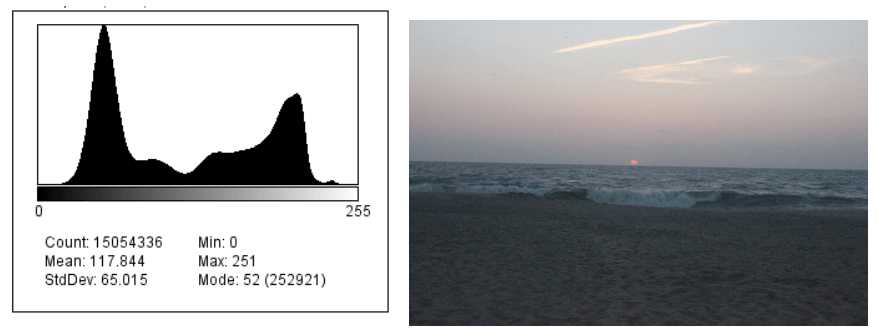
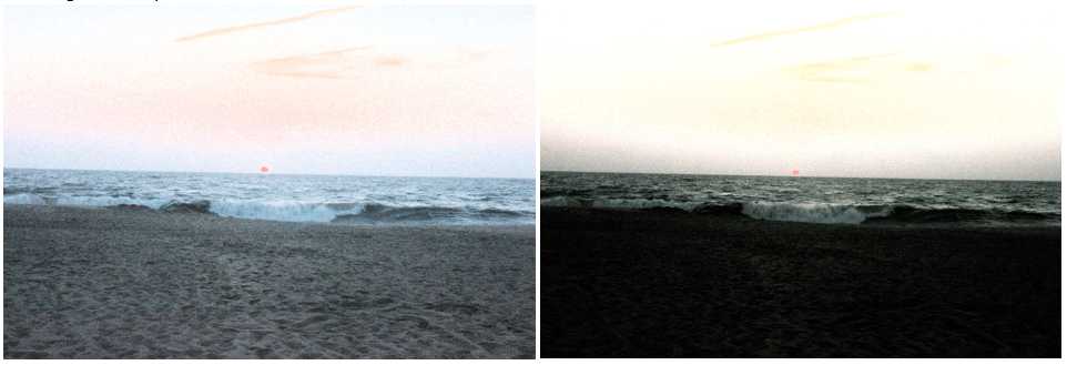
The beach scene featured above is an 8-bit jpeg image, which means that it has 2⁸ = 256 possible brightness levels, with 0 = completely black, and 255 = completely white.  Notice that this image has no completely black pixels (so the left hand side of the histogram shows zero value) nor any completely white pixels (so the right hand side also shows zero value).  The sand is fairly dark and accounts for the hump on the left side.  The sky is much lighter and its pixels are in the hump on the right side.  A fair degree of manipulation can be done with 8-bit images; but much more is possible with higher bit depth images.  Two examples of histogram manipulation for the beach scene are shown below:

Most high-end DSLRs will take 12 or 14 bit images, and specialized cameras will take 16+ bit images.  Usually specialized software is needed to make the most of these high bit depth images, though many standard programs such as Paint Shop Pro and Photoshop can do common tasks.  Such images have a much greater dynamic range, because they can cover more brightness levels.  For example, a 14 bit image contains not 256 brightness levels but 2¹⁴ = 16,384 brightness levels.  The human eye can only discern 256 or so levels, so many versions of the same image can be made by mapping different sets of the 16,384 brightness levels of the 14 bit image to 256 displayable levels.  How to do this in order to extract the desired information from an image is one of the challenges of digital image processing.  The starfield pair at the beginning of this article (which shows the aptly-name Crescent Nebula) demonstrates the possibilities.

Sharpening the Image

Much of image manipulation relies on the way that the human eye and visual system process information.  Take the following image and its sharpened version, using a technique that manipulates edge contrasts, effectively fooling the visual system into thinking that sharpness has increased:

Real sharpening of images is often a requirement.  Many techniques exist, some better than others and some not well-known but extremely effective.  Begin with the image on the left, which doesn’t look so bad. But, using a technique known as deconvolution, one can get the sharper image on the right.

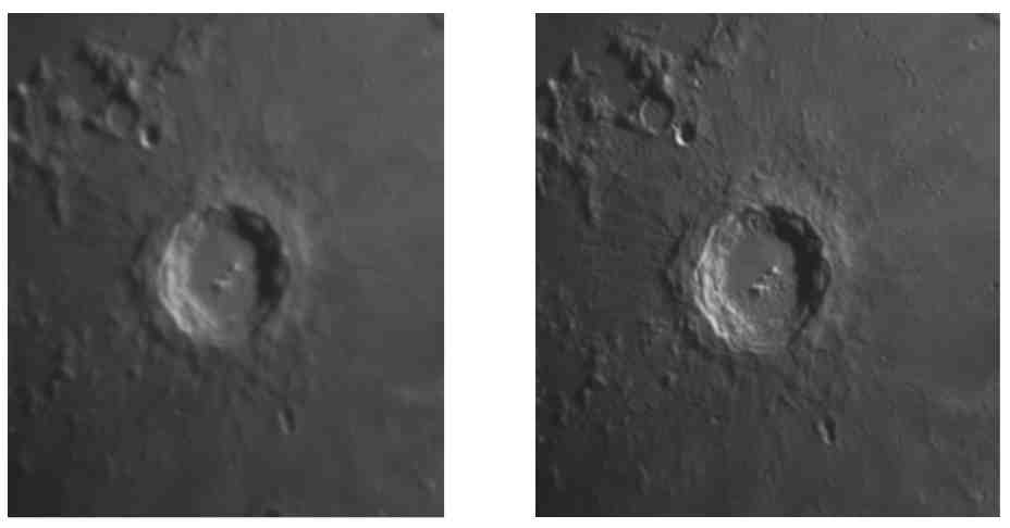
Ordinary sharpening methods will not produce this result, or anything close to it.  The technique is available in Photoshop (though buried) and some other image manipulation software, but almost no one knows about it.

Getting Rid of the Noise and Unwanted Backgrounds

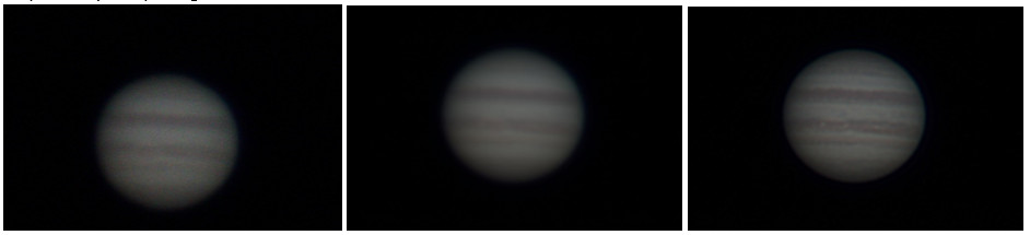
Noise is a common problem when imaging systems are pushed to their limits.  In digital images, noise is random pixel-to-pixel variations in brightness and color.  Noise can be reduced by image blurring, but better methods exist that leverage the mathematical fact that by averaging many images, signal-to-noise ratio can be significantly increased because the noise, being random, tends to cancel out whereas signal is strengthened.  The following three images show (1) a single shot of Jupiter; (2) the effect of “stacking” (averaging) many images; and (3) the result of using the above sharpening method on the stacked image.  If you look closely you can see that the noise, so readily apparent in the first image, is almost completely gone in the second.  This allows for sharpening of the second image; sharpening would not work on the first image because it is too noisy, and noise is amplified by sharpening methods.

How about removing unwanted backgrounds?  This is not so difficult using tools commonly available in most digital image processing  programs, including the freeware Gimp as well as Photoshop and Paint Shop Pro, though it is not a simple button push or mouse click.  See the example below.

Optical System Performance

Optical performance capabilities go hand-in-hand with digital image recording technology to determine overall image manipulation limits.  Any optical system is limited by the laws of physics, primarily diffraction; but all are the result of design compromises that reflect the goals of the optical system designers.  For example, in metrology, a certain degree of contrast is needed for accurate edge detection.  So how does one gauge optical capabilities?  There are different measures, depending on the application.  For example, is there an analogy to audio frequency response?  Fortunately, yes; it’s called the “Modulation Transfer Function” (MTF), and it is very useful for gauging how one optical system performs relative to another.  Analogous to audio systems, optical system performance deteriorates at “higher frequencies”, which in the case of the optical system correspond to imaging of closely spaced black and white bars.  As the bars get closer together, they tend to blur into each other, i.e., contrast decreases, ultimately leading to just a grey mass.  Here are two typical test images:

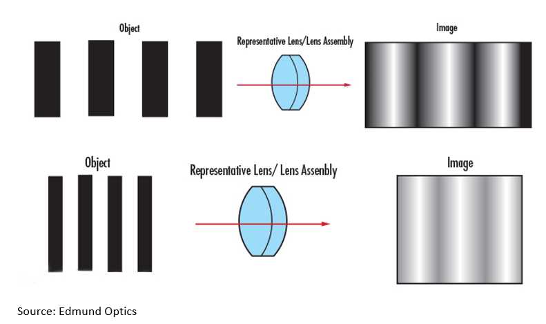
Source: Edmund Optics

Eventually, as the line pairs (bars) get smaller and closer together, one sees first what is below left, then what is below right:

The MTF measures the contrast between these bars, or “line pairs”, as they are called.  As the spatial frequency (number of line pairs or bars per millimeter) increases, contrast decreases, making discernment of the bars more difficult.  Here is an MTF plot for theoretically perfect optics:

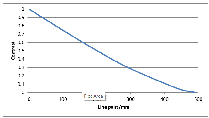
Units on the horizontal axis are line pairs per millimeter.  The vertical axis measures contrast.  When contrast drops to 0, no bars can be detected.  Most applications require the MTF to be 10% or higher.  Real imaging systems consist of several elements: lenses, filters, and detectors.  The MTF of the total system is, conveniently, the product of the MTFs of the individual elements.  Here is an example of using the MTF to compare the resolution of two types of telescopes:

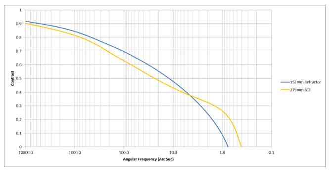
In this case, line pairs have been replaced by an equivalent measure more suited to telescopes, namely angular frequency (ability to distinguish objects separated by small angular distances), and the scale has been converted to logarithmic for clarity.

Digital Image Processing on the Job

By combining knowledge of optical system characteristics with knowledge of digital image capture and manipulation, you can achieve remarkable results, in many cases exceeding what was possible just a few years ago with film and film cameras.  If you are in a field that relies on image manipulation – for example, science, engineering, medicine, biology, robotics, geospatial imaging, intelligence, and forensics, among others – you will find the acquisition of the type of image processing know-how illustrated in this article to be well worth your effort. The Eogogics Digital Image Processing Training, a 1 to 3 day course, studies the principles, algorithms and technologies for acquiring, enhancing, transmitting, and analyzing digital images. Take a look.